Has anyone made a dumbbell dot plot in #rstats, or better yet exported to @plotlygraphs using the API? https://t.co/rWUSpH1rRl
— Ken Davis (@ken_mke) October 23, 2015
Last active
June 30, 2019 12:09
-
-
Save hrbrmstr/0d206070cea01bcb0118 to your computer and use it in GitHub Desktop.
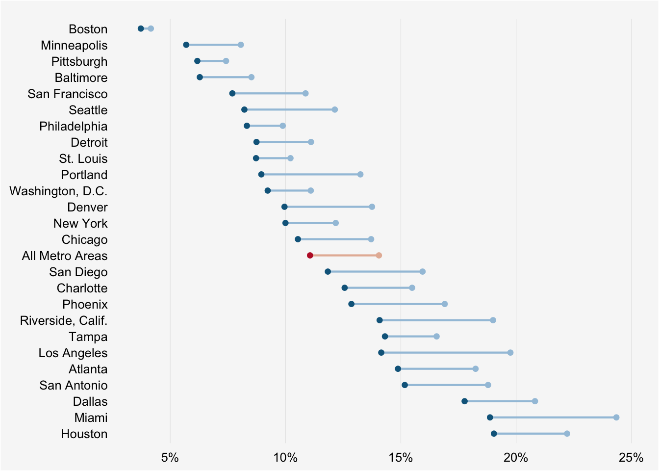
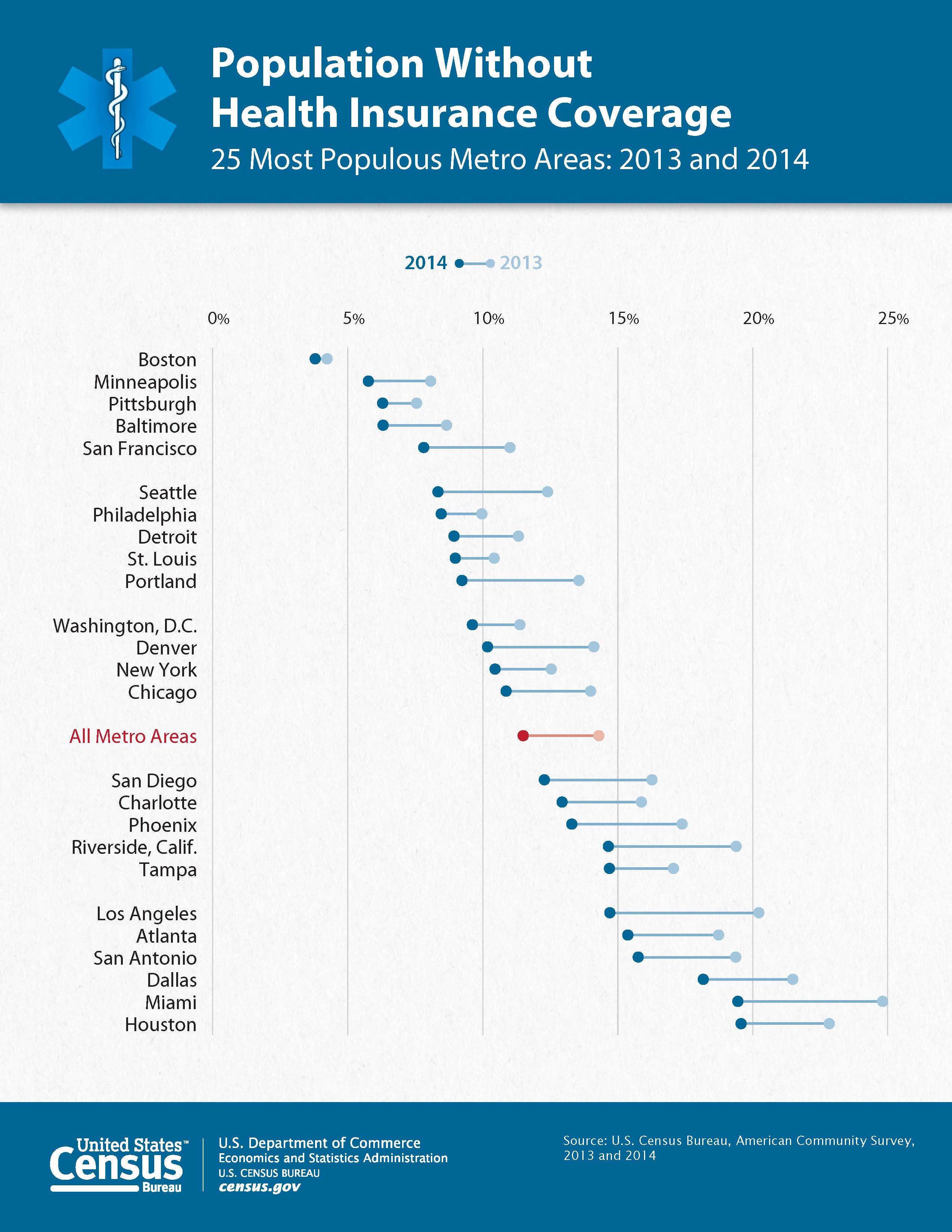
R+ggplot2 version of the "dumbbell" plot at http://census.gov/content/dam/Census/newsroom/releases/2015/cb15-158_graphic_acs_metro.jpg
This file contains hidden or bidirectional Unicode text that may be interpreted or compiled differently than what appears below. To review, open the file in an editor that reveals hidden Unicode characters.
Learn more about bidirectional Unicode characters
| area_id | area_name | |
|---|---|---|
| 0 | Houston | |
| 1 | Miami | |
| 2 | Dallas | |
| 3 | San Antonio | |
| 4 | Atlanta | |
| 5 | Los Angeles | |
| 7 | Tampa | |
| 8 | Riverside, Calif. | |
| 9 | Phoenix | |
| 10 | Charlotte | |
| 11 | San Diego | |
| 13 | All Metro Areas | |
| 15 | Chicago | |
| 16 | New York | |
| 17 | Denver | |
| 18 | Washington, D.C. | |
| 20 | Portland | |
| 21 | St. Louis | |
| 22 | Detroit | |
| 23 | Philadelphia | |
| 24 | Seattle | |
| 26 | San Francisco | |
| 27 | Baltimore | |
| 28 | Pittsburgh | |
| 29 | Minneapolis | |
| 30 | Boston |
This file contains hidden or bidirectional Unicode text that may be interpreted or compiled differently than what appears below. To review, open the file in an editor that reveals hidden Unicode characters.
Learn more about bidirectional Unicode characters
| 22.209907307969008 | 0.19674900165782105 | |
|---|---|---|
| 19.036743162789726 | 0.25618033761169556 | |
| 18.86689466056366 | 1.159849440615588 | |
| 24.347402225025796 | 1.3381434484772043 | |
| 17.766163759396925 | 2.2095945114639974 | |
| 20.81765006412328 | 2.3003054979199007 | |
| 15.171516750252842 | 3.251832466191914 | |
| 18.783221595470707 | 3.3453586211930073 | |
| 14.875767654756068 | 4.079492018475847 | |
| 18.24130165052289 | 4.32253490287669 | |
| 19.752108769771347 | 5.234649511516132 | |
| 14.151330949128862 | 5.281881783774203 | |
| 16.551887726907797 | 7.1783669937127925 | |
| 14.312421149214359 | 7.24249027724197 | |
| 14.080326142489234 | 8.145846583740841 | |
| 18.99920758218728 | 8.245941465347371 | |
| 12.856509816596983 | 9.270350019289118 | |
| 16.902532609035646 | 9.290681792115443 | |
| 12.563575889645392 | 10.248777486992886 | |
| 15.489161601101042 | 10.263478922728844 | |
| 11.834916431200408 | 11.225015379161505 | |
| 15.943185728138129 | 11.24565994849285 | |
| 14.050141279754765 | 13.195946157294934 | |
| 11.06371664807265 | 13.256315882763872 | |
| 10.537280130123342 | 15.06271569925659 | |
| 13.71325944384781 | 15.154052278722538 | |
| 9.998175353720711 | 16.190659896360096 | |
| 12.176803011187687 | 16.20160777403581 | |
| 13.75126421920779 | 17.189419136890177 | |
| 9.955635029037943 | 17.245722507793847 | |
| 9.226975570592955 | 18.221960399962466 | |
| 11.095778289837238 | 18.30672825282299 | |
| 8.950932654912467 | 20.104995360185175 | |
| 13.247349049619952 | 20.201962276741494 | |
| 8.721652816732526 | 21.159119582103873 | |
| 10.215568924709881 | 21.166626698224363 | |
| 11.105318583240361 | 22.15099729952351 | |
| 8.741358996548808 | 22.21449499004265 | |
| 8.323932060599105 | 23.192296864736363 | |
| 9.880094673075519 | 23.200116777361874 | |
| 8.216330062872094 | 24.096278764245277 | |
| 12.13785984631265 | 24.11598494406156 | |
| 7.694116297740564 | 26.12883045386773 | |
| 10.86868802719244 | 26.14478307562377 | |
| 8.52161945177199 | 27.112888258661858 | |
| 6.2821528740785535 | 27.177011542191035 | |
| 6.175958460624134 | 28.15637739940986 | |
| 7.420888550605261 | 28.162633329510268 | |
| 5.693469851630191 | 29.983098562178736 | |
| 8.061652191139517 | 29.14575274478933 | |
| 3.725510640294443 | 30.254616355086593 | |
| 4.16123617178784 | 30.256805930621738 |
This file contains hidden or bidirectional Unicode text that may be interpreted or compiled differently than what appears below. To review, open the file in an editor that reveals hidden Unicode characters.
Learn more about bidirectional Unicode characters
| # WebPlotDigitizer: http://arohatgi.info/WebPlotDigitizer/app/ | |
| library(dplyr) | |
| library(ggplot2) | |
| library(scales) | |
| health <- read.csv("health.csv", stringsAsFactors=FALSE, | |
| header=FALSE, col.names=c("pct", "area_id")) | |
| areas <- read.csv("area_trans.csv", stringsAsFactors=FALSE, header=TRUE) | |
| health %>% | |
| mutate(area_id=trunc(area_id)) %>% | |
| arrange(area_id, pct) %>% | |
| mutate(year=rep(c("2014", "2013"), 26), | |
| pct=pct/100) %>% | |
| left_join(areas, "area_id") %>% | |
| mutate(area_name=factor(area_name, levels=unique(area_name))) %>% | |
| mutate(color=rep(c("#0e668b", "#a3c4dc"), 26), | |
| line_col="#a3c4dc") -> health | |
| health[health$area_name=="All Metro Areas",]$color <- c("#bc1f31", "#e5b9a5") | |
| health[health$area_name=="All Metro Areas",]$line_col <- "#e5b9a5" | |
| gg <- ggplot(health) | |
| gg <- gg + geom_path(aes(x=pct, y=area_name, group=area_id, color=line_col), size=0.75) | |
| gg <- gg + geom_point(aes(x=pct, y=area_name, color=color), size=2.25) | |
| gg <- gg + scale_color_identity() | |
| gg <- gg + scale_x_continuous(label=percent) | |
| gg <- gg + labs(x=NULL, y=NULL) | |
| gg <- gg + theme_bw() | |
| gg <- gg + theme(plot.background=element_rect(fill="#f7f7f7")) | |
| gg <- gg + theme(panel.background=element_rect(fill="#f7f7f7")) | |
| gg <- gg + theme(panel.grid.minor=element_blank()) | |
| gg <- gg + theme(panel.grid.major.y=element_blank()) | |
| gg <- gg + theme(panel.grid.major.x=element_line()) | |
| gg <- gg + theme(axis.ticks=element_blank()) | |
| gg <- gg + theme(legend.position="top") | |
| gg <- gg + theme(panel.border=element_blank()) | |
| gg |
Sign up for free
to join this conversation on GitHub.
Already have an account?
Sign in to comment